CUR Decomposition: A low-rank approximation with column/row subsets

CUR approximation has become a popular topic in numerical linear algebra, and it has a particularly clean structure compared with other low-rank approximations. There are a few neat connections between CUR and other areas of numerical analysis as well: Yuji Nakatsukasa explained to me that polynomial interpolation can be viewed as CUR approximation; and the Nyström approximation (very popular in kernel methods) is a CUR approximation using a subsampling sketch. In this post, I hope to give a simple and intuitive explanation of this method, as well as why we might choose it over other low-rank methods in some situations.

Recap: Column subset selection

In our previous post, we introduced the column subset selection problem: the mathematics of how to choose representative columns from a large matrix. Given an $m \times n$ matrix $A$, we want to choose an $m\times r$ column submatrix of $A$, called $C$, so that the projection error $\|A-CC^\dagger A\|_F$ is as small as possible. Since $C$ contains the exact columns of $A$, it corresponds to choosing the representative data in applications, making it much easier to get a handle on than PCA/SVD. The number of columns $r$ is often small, like $5\sim20$, making it much easier to store and analyze than the whole matrix $A$.

Now, if $A$ represents measurements from experimental data, then we can do better than only selecting columns. For example, suppose $A$ is a table of gene-expression measurements from tumor samples. A column in $A$ would contain the gene measurements from one tumor specimen, and a row would contain measurements of a specific gene from different specimens. In this case, choosing both representative rows and columns would be of interest to a scientist and serves as one of the early motivations for CUR approximation [2].

What is CUR and how do we construct it?

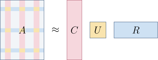
To define CUR, consider a column submatrix $C = A(:,J)$ and a row submatrix $R = A(I,:)$. Let $W = A(I,J)$ represent the intersection between $C$ and $R$. Then the CUR approximation is $A \approx C W^\dagger R = CUR$, where $U = W^\dagger$. As before, $^\dagger$ denotes the pseudoinverse. Note that $W$ is an $r\times r$ matrix, which is very small, so its pseudoinverse can be computed very quickly.

We construct the CUR approximation by applying column subset selection followed by row subset selection. Given a matrix $A$, we first select the column submatrix $C = A(:,J)$, with $J$ being the indices selected. We then apply column selection again on $C^T$, which gives us a row selection $I$. We are now ready to construct the CUR approximation:

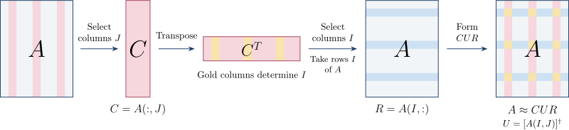
$C$ and $R$ are exact column and row submatrices of $A$, and $U = A(I,J)^\dagger$ is the pseudoinverse of the intersection between $C$ and $R$, known as the CUR core.

Why CUR instead of truncated SVD, randomised SVD, Nyström, etc.?

CUR is not a strictly better method than other popular low-rank methods, such as the ones listed in the title. In fact, there are many cases where CUR would be less accurate than those methods. However, CUR does have its own edge in some scenarios.

First of all, while approximating using only a few exact rows and columns might seem crude, CUR actually has surprisingly good approximation quality [3]. The key theorem¹ is the following: given ANY $m \times n$ matrix $A$, let $A_r$ be the best rank-$r$ approximation to $A$²; then there exists a rank-$r$ CUR approximation such that

$$\|A-CUR\|_F \leq (r+1)\| A - A_r\|_F.$$

As before, $r$ is the number of columns/rows used and is quite small, e.g., around $5\sim 20$. Therefore, CUR can achieve an accuracy quite close to the optimal approximation, even though many other methods would require the entire matrix and CUR only requires a small column/row subset³.

The structure of CUR makes it particularly easy to update. For example, if we already have $A\approx CUR$ and now we append an additional column to $A$, we can often keep the same $C$ and $U$, while just updating $R$ to include the new column. This quick update would not be as fast if you used SVD instead.

Preserving sparsity is also a good motivation. In many applications, $A$ is very sparse, i.e., it contains a lot of 0s. If you apply SVD to $A$, the resulting decomposition is likely dense and does not contain a lot of 0s. However, as $C$ and $R$ are the exact data from $A$, they could potentially both be as sparse as $A$ is. Modern matrix operations are often optimized for sparsity, and using CUR can make use of these optimizations.

Tips and tricks when applying CUR

In the final section, I want to give some tips and tricks for implementing CUR for approximating matrices. These tips are not exhaustive and often come from my own coding experiences.

1. Is there low-rank structure? CUR is ultimately a low-rank approximation method; therefore, it is necessary to have sufficient decay in the singular values.
2. Pivoting methods: The previous blog has a short section on which methods are available to select the columns and rows. It should also be said that it is important to select rows based on the existing columns, not the entire matrix $A$.
3. Truncate the core: If CUR is not as accurate as you hope for, in many cases the issue is not the CUR itself, but the numerical error from the ill-conditioning of $A(I,J)$. Specifically, if the minimum singular value of $A(I,J)$ is too small, taking the pseudoinverse might create a large numerical error in computation. An easy fix is to instead truncate the singular values of $A(I,J)$ that are less than some $\epsilon$, say $\epsilon = 10^{-15}$ for a suitably scaled matrix⁴. [1] is a great reference if you want to have a better understanding of the $\epsilon$-pseudoinverse.
4. Oversampling: Another useful tip from [1] is oversampling, which means choosing a few more rows than your target column rank. This can be understood to improve your approximation in two ways: first, oversampling incorporates more row information; secondly, oversampling can improve the core conditioning.

References

1. Park, T. and Nakatsukasa, Y., 2025. Accuracy and stability of CUR decompositions with oversampling. SIAM Journal on Matrix Analysis and Applications, 46(1), pp.780-810.
2. Mahoney, M.W. and Drineas, P., 2009. CUR matrix decompositions for improved data analysis. Proceedings of the National Academy of Sciences, 106(3), pp.697-702.
3. Zamarashkin, N.L. and Osinsky, A.I., 2018, March. On the existence of a nearly optimal skeleton approximation of a matrix in the Frobenius norm. In Doklady Mathematics (Vol. 97, No. 2, pp. 164-166). Moscow: Pleiades Publishing.

Footnotes

1. which is sometimes known as the Fundamental Theorem of CUR ↩

2. i.e., the truncated SVD ↩

3. Given good pivots. ↩

4. Concretely, let $A(I,J) = U\Sigma V^T$ be its economy-size SVD; then $A(I,J)^\dagger = V\Sigma^{-1} U^T$. The $\epsilon$-pseudoinverse inverts only the entries of $\Sigma$ that are greater than $\epsilon$ and sets the rest to $0$. ↩