How can polynomial interpolation remove noise? (Part I)

This blog post is based on the work of Takeru Matsuda and my mentor, Yuji Nakatsukasa. In their paper Polynomial approximation of noisy functions, they developed a surprisingly simple yet powerful method for approximating noisy functions, called NoisyChebtrunc.

If you are given an unknown (sufficiently smooth) function $f(x)$, say on $[-1,1]$, and all you can do is sample $f$ at points of your choice, $x_0, x_1, \dots, x_N$, how will you go about approximating (or learning) $f$? At least to me, there are two different approaches depending on your taste.

Two approaches

Numerical analysts: We should take samples at the famous Chebyshev points

$$x_i = \cos\left(\frac{i\pi}{N}\right)$$

and find the unique degree-$N$ polynomial $p_N$ that goes through all $N+1$ sample points.

Statisticians: We should take $N+1$ samples (randomly or deterministically) and use least-squares to fit the samples to a polynomial of degree $n\leq N$.

The numerical analysts’ approach has several computational advantages: Chebyshev interpolation has a near-best convergence guarantee, can be performed in $O(N\log N)$ time, and can be computed stably using the fast Fourier transform (FFT).¹

Why interpolation struggles with noise

Suppose the samples are not exact but instead noisy, as they always are in real life:

$$y_i = f(x_i) + \epsilon,$$

where $\epsilon$ is a noise term. An interpolation approach quickly becomes problematic: an interpolant $p_N$ passes through all the samples $(x_i,y_i)$ by definition, so you have no hope of recovering the true $f(x_i)$. In fact, even a small amount of noise can magnify the approximation error.

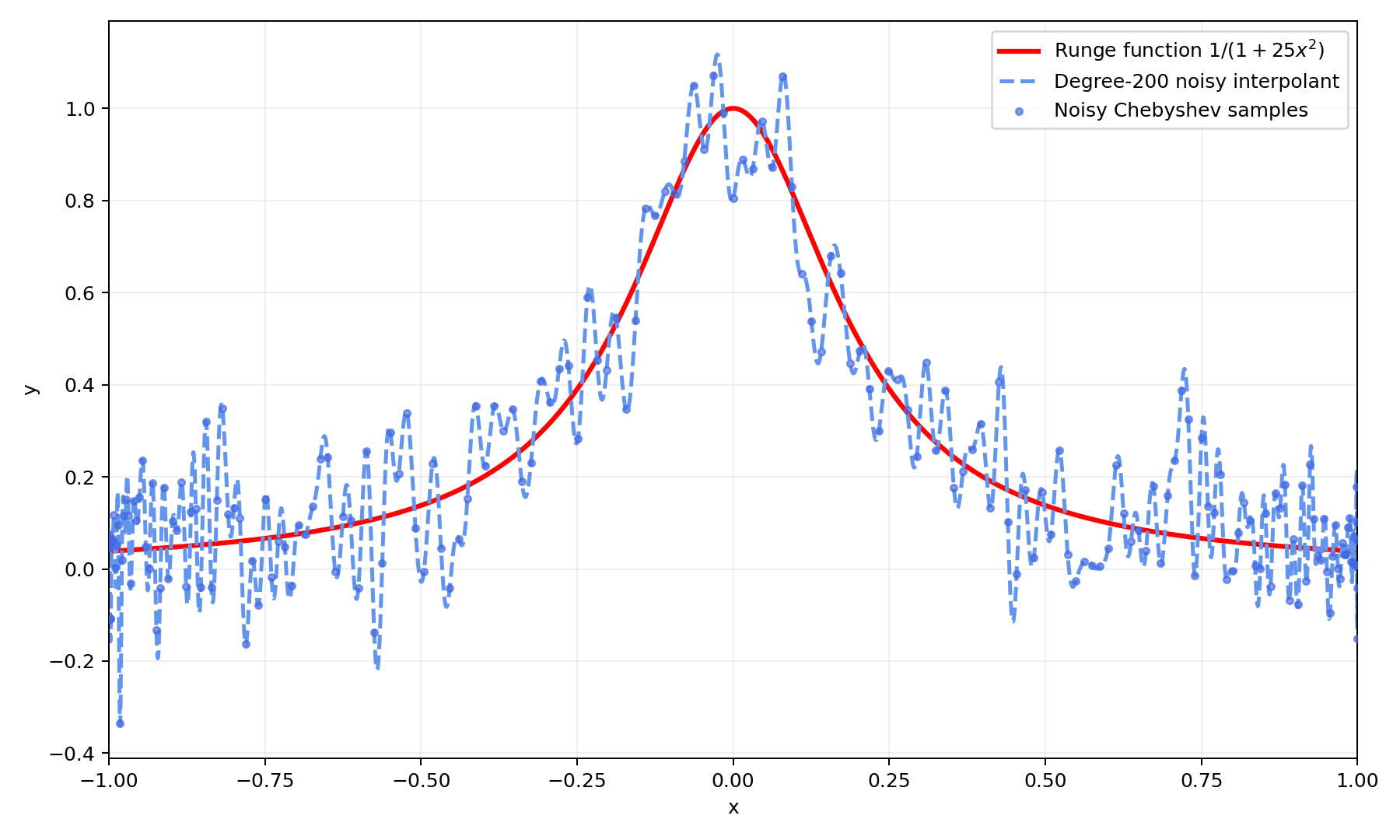
By contrast, least-squares is much more robust to noise provided a suitable degree $n$ is chosen. It can reduce the noise at a rate of $O(1/\sqrt{N})$.

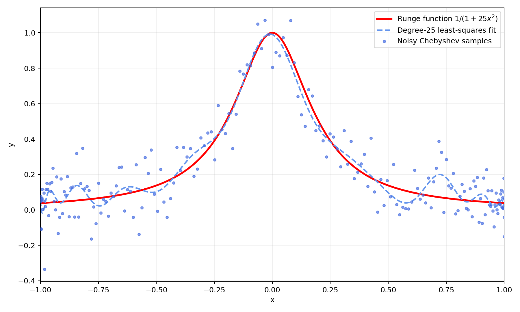
It might be counter-intuitive, or at least it certainly was to me, that a lower-degree polynomial would achieve a better approximation. This is essentially explained by polynomial overfitting; see Larry Wasserman’s All of Statistics.

The interpolation approach certainly has its virtues, but the high-order oscillations make it noise-sensitive, which is very undesirable in the real world. Is there a quick fix we can apply to $p_N$ to remove them?

Truncating the high-order terms

It turns out there is: just truncate the high-order terms! The higher-order coefficients of $p_N$ are typically small and somehow “carry” the noisy oscillations in the approximation. Think of the Fourier series, where the higher-order terms contain higher frequencies and hence more oscillations.²

Therefore, if we choose some small $n$ and simply chop off the terms of $p_N$ to get a degree-$n$ polynomial $\tilde{p}_n$, we can remove oscillations and hopefully recover $f$ with less noise.

The mathematics, of course, is more complicated. The most obvious question is: how should $n$ be selected? The answer is to learn from the statisticians and see how they would select such a degree: Mallows’ $C_p$.

Choosing the degree with Mallows’ criterion

Let

$$p_N = \sum_{j=0}^{N} c_j T_j,$$

where $T_j$ is the $j$th Chebyshev polynomial and $c_j$ is the corresponding coefficient. We define

$$\begin{aligned} C_p(\ell) \approx {}& \underbrace{\frac{N}{2}\sum_{j>\ell} \lvert c_j\rvert^2}_{\text{information discarded}} \\ &+ \underbrace{2\hat{\sigma}^2(\ell+1)}_{\text{cost of keeping coefficients}}. \end{aligned}$$

We choose the truncation degree to minimize the $C_p$ value:

$$n = \operatorname*{arg\,min}_{\ell} C_p(\ell).$$

Here $\hat{\sigma}$ is an estimator of the standard deviation of the noise based on the samples.

The idea is a balancing act between keeping more information about the underlying $f$ and removing noise. The first term measures the size of the truncated coefficients, representing the amount of “knowledge” of $f$ removed by truncating at degree $\ell$. The latter term increases with $\ell$, controlling polynomial overfitting and the noise contained in the kept terms.

Therefore, by truncating at $n$ with the smallest $C_p$, we can remove the effect of noise from the high-order terms while retaining enough information about $f$ in the kept terms.

The NoisyChebtrunc algorithm

We are now ready to unveil the final algorithm, NoisyChebtrunc. It has, as the name suggests, three steps:

1. Noisy: Take $N+1$ noisy samples at the Chebyshev points.
2. Cheb: Apply Chebyshev interpolation to the samples to compute the degree-$N$ interpolant $p_N$, using the FFT/DCT.
3. trunc: Truncate $p_N$ at the degree $n$ selected via $C_p$, yielding the output $\hat{p}_n$.

How good is NoisyChebtrunc in practice? It has the best of both worlds: the speed and stability of Chebyshev interpolation and the $O(1/\sqrt{N})$ denoising effect of least-squares. Here is NoisyChebtrunc applied to the same example with 201 sample points—voilà!

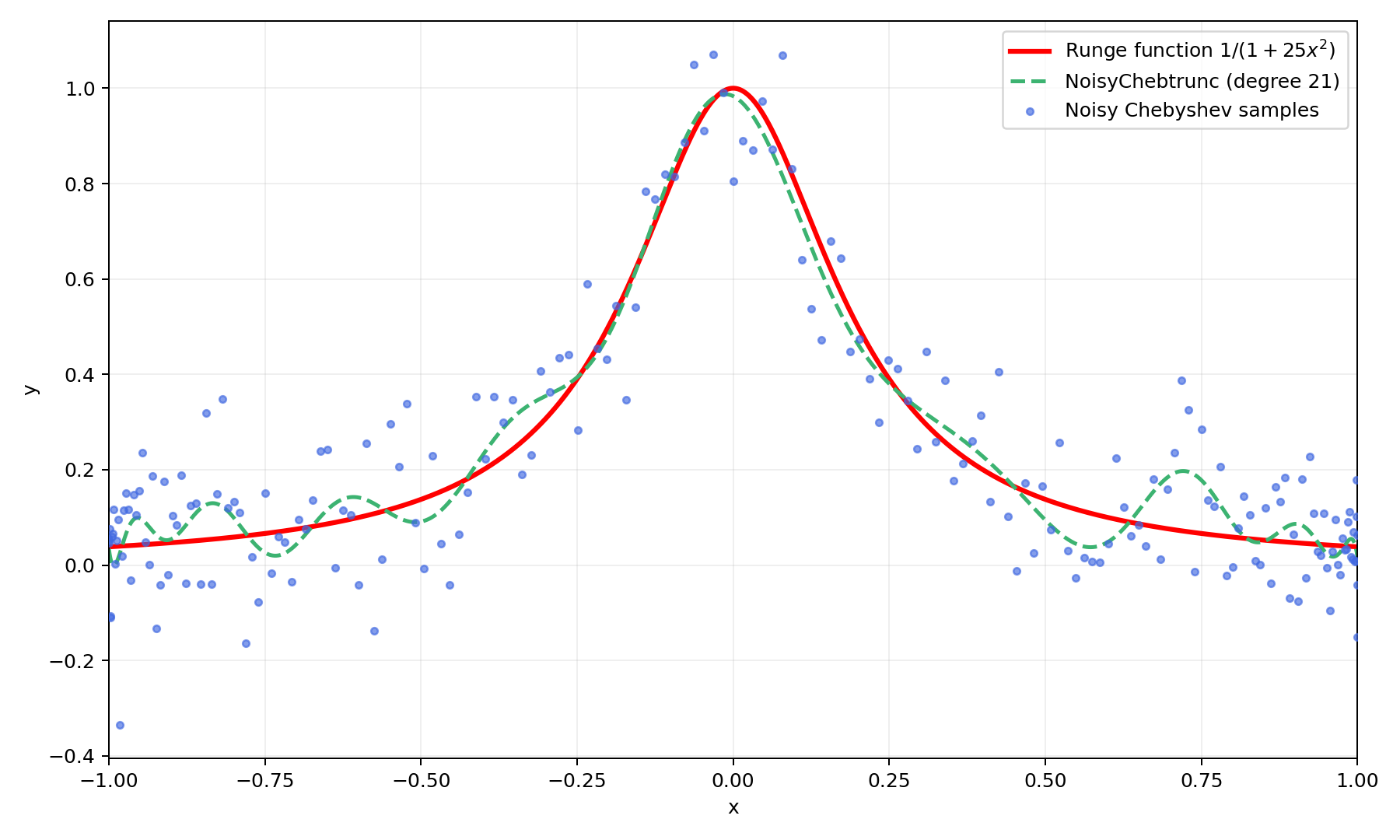
The truncated interpolant fits the original $f$ much better than the plain interpolant does, with accuracy similar to that of the least-squares solution.³

Before you go

Interpolation is one of the most common tools in the repertoire of a computational mathematician. If your interpolants are not behaving well due to noisy samples, a simple but effective trick is to truncate to a much smaller degree $n$, and Mallows’ $C_p$ gives a good way to choose $n$.

References

1. T. Matsuda and Y. Nakatsukasa, “Polynomial approximation of noisy functions”, Numerische Mathematik 157 (2025), 1285–1311.
2. L. Wasserman, All of Statistics: A Concise Course in Statistical Inference, Springer, 2004.
3. L. N. Trefethen, Approximation Theory and Approximation Practice, Extended Edition, SIAM, 2019.

Footnotes

1. If you want to know more about the amazing properties of the FFT and Chebyshev interpolation, please check out Ethan Epperly’s (much better written) post, “Chebyshev Polynomials and Chebyshev Interpolation”. ↩

2. This is no surprise to readers familiar with the connection between Chebyshev interpolation and Fourier series. See Lloyd N. Trefethen’s Approximation Theory and Approximation Practice, Extended Edition. ↩

3. In fact, Matsuda and Nakatsukasa showed that NoisyChebtrunc can be viewed as weighted least-squares; they then applied this insight to prove high-probability convergence guarantees. ↩